TorchVision Object Detection Finetuning Tutorial

For this tutorial, we will be finetuning a pre-trained Mask R-CNN model on the Penn-Fudan Database for Pedestrian Detection and Segmentation. It contains 170 images with 345 instances of pedestrians, and we will use it to illustrate how to use the new features in torchvision in order to train an object detection and instance segmentation model on a custom dataset.

Note

This tutorial works only with torchvision version >=0.16 or nightly. If you’re using torchvision<=0.15, please follow this tutorial instead.

Defining the Dataset

The reference scripts for training object detection, instance segmentation and person keypoint detection allows for easily supporting adding new custom datasets. The dataset should inherit from the standard torch.utils.data.Dataset class, and implement __len__ and __getitem__.

The only specificity that we require is that the dataset __getitem__ should return a tuple:

• image: torchvision.tv_tensors.Image of shape [3, H, W], a pure tensor, or a PIL Image of size (H, W)

• target: a dict containing the following fields

  • boxes, torchvision.tv_tensors.BoundingBoxes of shape [N, 4]: the coordinates of the N bounding boxes in [x0, y0, x1, y1] format, ranging from 0 to W and 0 to H

  • labels, integer torch.Tensor of shape [N]: the label for each bounding box. 0 represents always the background class.

  • image_id, int: an image identifier. It should be unique between all the images in the dataset, and is used during evaluation

  • area, float torch.Tensor of shape [N]: the area of the bounding box. This is used during evaluation with the COCO metric, to separate the metric scores between small, medium and large boxes.

  • iscrowd, uint8 torch.Tensor of shape [N]: instances with iscrowd=True will be ignored during evaluation.

  • (optionally) masks, torchvision.tv_tensors.Mask of shape [N, H, W]: the segmentation masks for each one of the objects

If your dataset is compliant with above requirements then it will work for both training and evaluation codes from the reference script. Evaluation code will use scripts from pycocotools which can be installed with pip install pycocotools.

Note

For Windows, please install pycocotools from gautamchitnis with command

pip install git+https://github.com/gautamchitnis/cocoapi.git@cocodataset-master#subdirectory=PythonAPI

One note on the labels. The model considers class 0 as background. If your dataset does not contain the background class, you should not have 0 in your labels. For example, assuming you have just two classes, cat and dog, you can define 1 (not 0) to represent cats and 2 to represent dogs. So, for instance, if one of the images has both classes, your labels tensor should look like [1, 2].

Additionally, if you want to use aspect ratio grouping during training (so that each batch only contains images with similar aspect ratios), then it is recommended to also implement a get_height_and_width method, which returns the height and the width of the image. If this method is not provided, we query all elements of the dataset via __getitem__ , which loads the image in memory and is slower than if a custom method is provided.

Writing a custom dataset for PennFudan

Let’s write a dataset for the PennFudan dataset. First, let’s download the dataset and extract the zip file:

wget https://www.cis.upenn.edu/~jshi/ped_html/PennFudanPed.zip -P data
cd data && unzip PennFudanPed.zip

We have the following folder structure:

PennFudanPed/
  PedMasks/
    FudanPed00001_mask.png
    FudanPed00002_mask.png
    FudanPed00003_mask.png
    FudanPed00004_mask.png
    ...
  PNGImages/
    FudanPed00001.png
    FudanPed00002.png
    FudanPed00003.png
    FudanPed00004.png

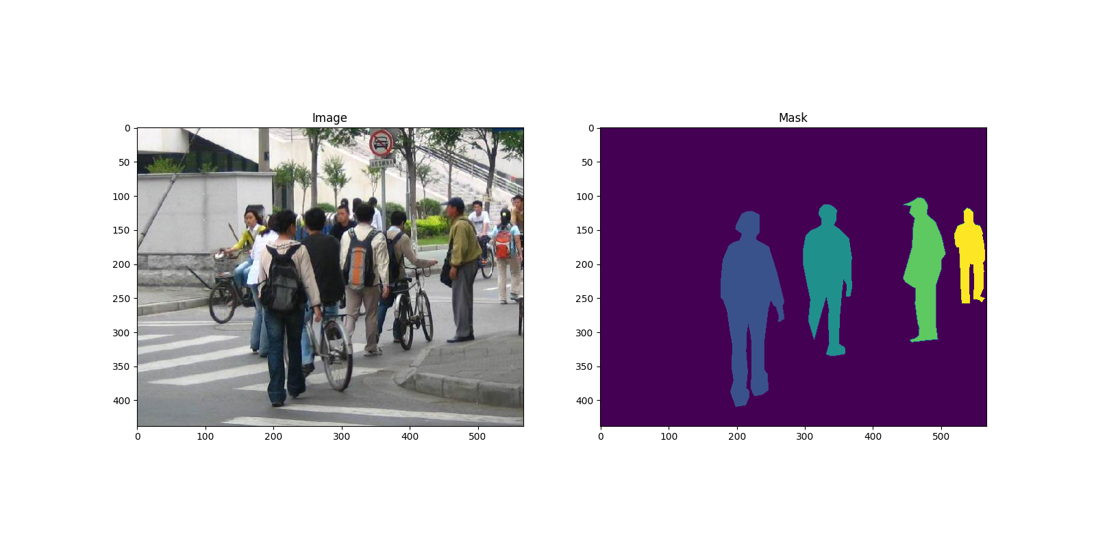
Here is one example of a pair of images and segmentation masks

import matplotlib.pyplot as plt
from torchvision.io import read_image


image = read_image("data/PennFudanPed/PNGImages/FudanPed00046.png")
mask = read_image("data/PennFudanPed/PedMasks/FudanPed00046_mask.png")

plt.figure(figsize=(16, 8))
plt.subplot(121)
plt.title("Image")
plt.imshow(image.permute(1, 2, 0))
plt.subplot(122)
plt.title("Mask")
plt.imshow(mask.permute(1, 2, 0))

<matplotlib.image.AxesImage object at 0x7f8258082260>

So each image has a corresponding segmentation mask, where each color correspond to a different instance. Let’s write a torch.utils.data.Dataset class for this dataset. In the code below, we are wrapping images, bounding boxes and masks into torchvision.tv_tensors.TVTensor classes so that we will be able to apply torchvision built-in transformations (new Transforms API) for the given object detection and segmentation task. Namely, image tensors will be wrapped by torchvision.tv_tensors.Image, bounding boxes into torchvision.tv_tensors.BoundingBoxes and masks into torchvision.tv_tensors.Mask. As torchvision.tv_tensors.TVTensor are torch.Tensor subclasses, wrapped objects are also tensors and inherit the plain torch.Tensor API. For more information about torchvision tv_tensors see this documentation.

import os
import torch

from torchvision.io import read_image
from torchvision.ops.boxes import masks_to_boxes
from torchvision import tv_tensors
from torchvision.transforms.v2 import functional as F


class PennFudanDataset(torch.utils.data.Dataset):
    def __init__(self, root, transforms):
        self.root = root
        self.transforms = transforms
        # load all image files, sorting them to
        # ensure that they are aligned
        self.imgs = list(sorted(os.listdir(os.path.join(root, "PNGImages"))))
        self.masks = list(sorted(os.listdir(os.path.join(root, "PedMasks"))))

    def __getitem__(self, idx):
        # load images and masks
        img_path = os.path.join(self.root, "PNGImages", self.imgs[idx])
        mask_path = os.path.join(self.root, "PedMasks", self.masks[idx])
        img = read_image(img_path)
        mask = read_image(mask_path)
        # instances are encoded as different colors
        obj_ids = torch.unique(mask)
        # first id is the background, so remove it
        obj_ids = obj_ids[1:]
        num_objs = len(obj_ids)

        # split the color-encoded mask into a set
        # of binary masks
        masks = (mask == obj_ids[:, None, None]).to(dtype=torch.uint8)

        # get bounding box coordinates for each mask
        boxes = masks_to_boxes(masks)

        # there is only one class
        labels = torch.ones((num_objs,), dtype=torch.int64)

        image_id = idx
        area = (boxes[:, 3] - boxes[:, 1]) * (boxes[:, 2] - boxes[:, 0])
        # suppose all instances are not crowd
        iscrowd = torch.zeros((num_objs,), dtype=torch.int64)

        # Wrap sample and targets into torchvision tv_tensors:
        img = tv_tensors.Image(img)

        target = {}
        target["boxes"] = tv_tensors.BoundingBoxes(boxes, format="XYXY", canvas_size=F.get_size(img))
        target["masks"] = tv_tensors.Mask(masks)
        target["labels"] = labels
        target["image_id"] = image_id
        target["area"] = area
        target["iscrowd"] = iscrowd

        if self.transforms is not None:
            img, target = self.transforms(img, target)

        return img, target

    def __len__(self):
        return len(self.imgs)

That’s all for the dataset. Now let’s define a model that can perform predictions on this dataset.

Defining your model

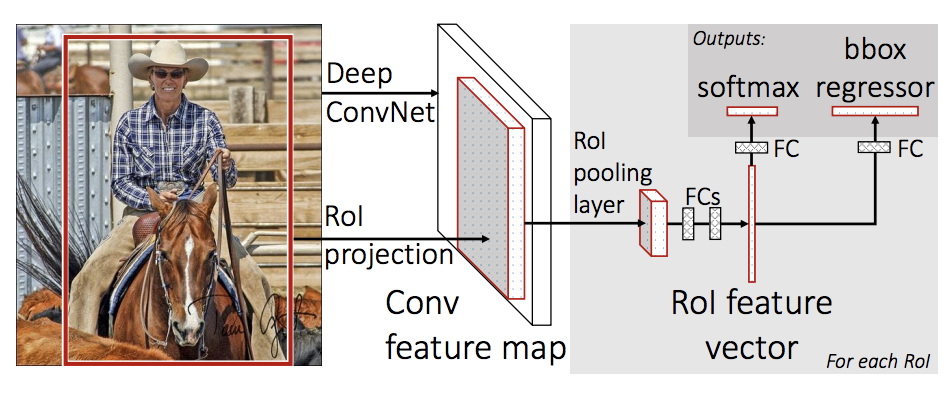
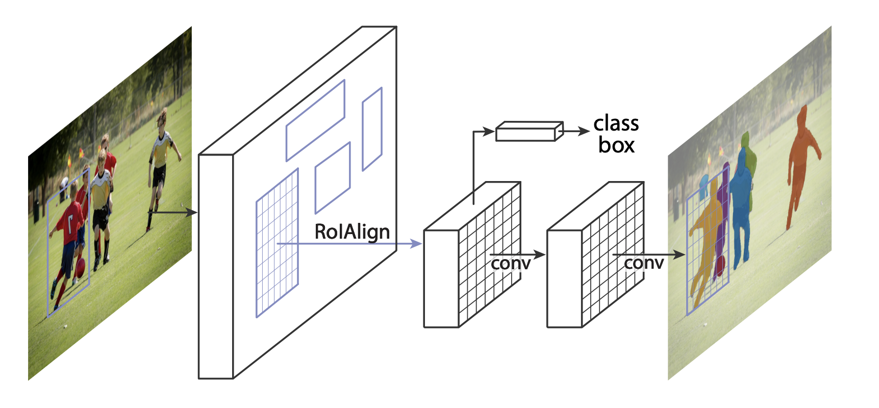
In this tutorial, we will be using Mask R-CNN, which is based on top of Faster R-CNN. Faster R-CNN is a model that predicts both bounding boxes and class scores for potential objects in the image.

Mask R-CNN adds an extra branch into Faster R-CNN, which also predicts segmentation masks for each instance.

There are two common situations where one might want to modify one of the available models in TorchVision Model Zoo. The first is when we want to start from a pre-trained model, and just finetune the last layer. The other is when we want to replace the backbone of the model with a different one (for faster predictions, for example).

Let’s go see how we would do one or another in the following sections.

1 - Finetuning from a pretrained model

Let’s suppose that you want to start from a model pre-trained on COCO and want to finetune it for your particular classes. Here is a possible way of doing it:

import torchvision
from torchvision.models.detection.faster_rcnn import FastRCNNPredictor

# load a model pre-trained on COCO
model = torchvision.models.detection.fasterrcnn_resnet50_fpn(weights="DEFAULT")

# replace the classifier with a new one, that has
# num_classes which is user-defined
num_classes = 2  # 1 class (person) + background
# get number of input features for the classifier
in_features = model.roi_heads.box_predictor.cls_score.in_features
# replace the pre-trained head with a new one
model.roi_heads.box_predictor = FastRCNNPredictor(in_features, num_classes)

Downloading: "https://download.pytorch.org/models/fasterrcnn_resnet50_fpn_coco-258fb6c6.pth" to /var/lib/ci-user/.cache/torch/hub/checkpoints/fasterrcnn_resnet50_fpn_coco-258fb6c6.pth

  0%|          | 0.00/160M [00:00<?, ?B/s]
 19%|#8        | 29.8M/160M [00:00<00:00, 312MB/s]
 37%|###7      | 59.5M/160M [00:00<00:00, 263MB/s]
 59%|#####9    | 95.0M/160M [00:00<00:00, 308MB/s]
 78%|#######8  | 125M/160M [00:00<00:00, 306MB/s]
 97%|#########6| 155M/160M [00:00<00:00, 282MB/s]
100%|##########| 160M/160M [00:00<00:00, 286MB/s]

2 - Modifying the model to add a different backbone

import torchvision
from torchvision.models.detection import FasterRCNN
from torchvision.models.detection.rpn import AnchorGenerator

# load a pre-trained model for classification and return
# only the features
backbone = torchvision.models.mobilenet_v2(weights="DEFAULT").features
# ``FasterRCNN`` needs to know the number of
# output channels in a backbone. For mobilenet_v2, it's 1280
# so we need to add it here
backbone.out_channels = 1280

# let's make the RPN generate 5 x 3 anchors per spatial
# location, with 5 different sizes and 3 different aspect
# ratios. We have a Tuple[Tuple[int]] because each feature
# map could potentially have different sizes and
# aspect ratios
anchor_generator = AnchorGenerator(
    sizes=((32, 64, 128, 256, 512),),
    aspect_ratios=((0.5, 1.0, 2.0),)
)

# let's define what are the feature maps that we will
# use to perform the region of interest cropping, as well as
# the size of the crop after rescaling.
# if your backbone returns a Tensor, featmap_names is expected to
# be [0]. More generally, the backbone should return an
# ``OrderedDict[Tensor]``, and in ``featmap_names`` you can choose which
# feature maps to use.
roi_pooler = torchvision.ops.MultiScaleRoIAlign(
    featmap_names=['0'],
    output_size=7,
    sampling_ratio=2
)

# put the pieces together inside a Faster-RCNN model
model = FasterRCNN(
    backbone,
    num_classes=2,
    rpn_anchor_generator=anchor_generator,
    box_roi_pool=roi_pooler
)

Downloading: "https://download.pytorch.org/models/mobilenet_v2-7ebf99e0.pth" to /var/lib/ci-user/.cache/torch/hub/checkpoints/mobilenet_v2-7ebf99e0.pth

  0%|          | 0.00/13.6M [00:00<?, ?B/s]
 81%|########  | 11.0M/13.6M [00:00<00:00, 115MB/s]
100%|##########| 13.6M/13.6M [00:00<00:00, 110MB/s]

Object detection and instance segmentation model for PennFudan Dataset

In our case, we want to finetune from a pre-trained model, given that our dataset is very small, so we will be following approach number 1.

Here we want to also compute the instance segmentation masks, so we will be using Mask R-CNN:

import torchvision
from torchvision.models.detection.faster_rcnn import FastRCNNPredictor
from torchvision.models.detection.mask_rcnn import MaskRCNNPredictor


def get_model_instance_segmentation(num_classes):
    # load an instance segmentation model pre-trained on COCO
    model = torchvision.models.detection.maskrcnn_resnet50_fpn(weights="DEFAULT")

    # get number of input features for the classifier
    in_features = model.roi_heads.box_predictor.cls_score.in_features
    # replace the pre-trained head with a new one
    model.roi_heads.box_predictor = FastRCNNPredictor(in_features, num_classes)

    # now get the number of input features for the mask classifier
    in_features_mask = model.roi_heads.mask_predictor.conv5_mask.in_channels
    hidden_layer = 256
    # and replace the mask predictor with a new one
    model.roi_heads.mask_predictor = MaskRCNNPredictor(
        in_features_mask,
        hidden_layer,
        num_classes
    )

    return model

That’s it, this will make model be ready to be trained and evaluated on your custom dataset.

Putting everything together

In references/detection/, we have a number of helper functions to simplify training and evaluating detection models. Here, we will use references/detection/engine.py and references/detection/utils.py. Just download everything under references/detection to your folder and use them here. On Linux if you have wget, you can download them using below commands:

os.system("wget https://raw.githubusercontent.com/pytorch/vision/main/references/detection/engine.py")
os.system("wget https://raw.githubusercontent.com/pytorch/vision/main/references/detection/utils.py")
os.system("wget https://raw.githubusercontent.com/pytorch/vision/main/references/detection/coco_utils.py")
os.system("wget https://raw.githubusercontent.com/pytorch/vision/main/references/detection/coco_eval.py")
os.system("wget https://raw.githubusercontent.com/pytorch/vision/main/references/detection/transforms.py")

0

Since v0.15.0 torchvision provides new Transforms API to easily write data augmentation pipelines for Object Detection and Segmentation tasks.

Let’s write some helper functions for data augmentation / transformation:

from torchvision.transforms import v2 as T


def get_transform(train):
    transforms = []
    if train:
        transforms.append(T.RandomHorizontalFlip(0.5))
    transforms.append(T.ToDtype(torch.float, scale=True))
    transforms.append(T.ToPureTensor())
    return T.Compose(transforms)

Testing forward() method (Optional)

Before iterating over the dataset, it’s good to see what the model expects during training and inference time on sample data.

import utils

model = torchvision.models.detection.fasterrcnn_resnet50_fpn(weights="DEFAULT")
dataset = PennFudanDataset('data/PennFudanPed', get_transform(train=True))
data_loader = torch.utils.data.DataLoader(
    dataset,
    batch_size=2,
    shuffle=True,
    collate_fn=utils.collate_fn
)

# For Training
images, targets = next(iter(data_loader))
images = list(image for image in images)
targets = [{k: v for k, v in t.items()} for t in targets]
output = model(images, targets)  # Returns losses and detections
print(output)

# For inference
model.eval()
x = [torch.rand(3, 300, 400), torch.rand(3, 500, 400)]
predictions = model(x)  # Returns predictions
print(predictions[0])

{'loss_classifier': tensor(0.0798, grad_fn=<NllLossBackward0>), 'loss_box_reg': tensor(0.0284, grad_fn=<DivBackward0>), 'loss_objectness': tensor(0.0186, grad_fn=<BinaryCrossEntropyWithLogitsBackward0>), 'loss_rpn_box_reg': tensor(0.0034, grad_fn=<DivBackward0>)}
{'boxes': tensor([], size=(0, 4), grad_fn=<StackBackward0>), 'labels': tensor([], dtype=torch.int64), 'scores': tensor([], grad_fn=<IndexBackward0>)}

Let’s now write the main function which performs the training and the validation:

from engine import train_one_epoch, evaluate

# train on the GPU or on the CPU, if a GPU is not available
device = torch.device('cuda') if torch.cuda.is_available() else torch.device('cpu')

# our dataset has two classes only - background and person
num_classes = 2
# use our dataset and defined transformations
dataset = PennFudanDataset('data/PennFudanPed', get_transform(train=True))
dataset_test = PennFudanDataset('data/PennFudanPed', get_transform(train=False))

# split the dataset in train and test set
indices = torch.randperm(len(dataset)).tolist()
dataset = torch.utils.data.Subset(dataset, indices[:-50])
dataset_test = torch.utils.data.Subset(dataset_test, indices[-50:])

# define training and validation data loaders
data_loader = torch.utils.data.DataLoader(
    dataset,
    batch_size=2,
    shuffle=True,
    collate_fn=utils.collate_fn
)

data_loader_test = torch.utils.data.DataLoader(
    dataset_test,
    batch_size=1,
    shuffle=False,
    collate_fn=utils.collate_fn
)

# get the model using our helper function
model = get_model_instance_segmentation(num_classes)

# move model to the right device
model.to(device)

# construct an optimizer
params = [p for p in model.parameters() if p.requires_grad]
optimizer = torch.optim.SGD(
    params,
    lr=0.005,
    momentum=0.9,
    weight_decay=0.0005
)

# and a learning rate scheduler
lr_scheduler = torch.optim.lr_scheduler.StepLR(
    optimizer,
    step_size=3,
    gamma=0.1
)

# let's train it just for 2 epochs
num_epochs = 2

for epoch in range(num_epochs):
    # train for one epoch, printing every 10 iterations
    train_one_epoch(model, optimizer, data_loader, device, epoch, print_freq=10)
    # update the learning rate
    lr_scheduler.step()
    # evaluate on the test dataset
    evaluate(model, data_loader_test, device=device)

print("That's it!")

Downloading: "https://download.pytorch.org/models/maskrcnn_resnet50_fpn_coco-bf2d0c1e.pth" to /var/lib/ci-user/.cache/torch/hub/checkpoints/maskrcnn_resnet50_fpn_coco-bf2d0c1e.pth

  0%|          | 0.00/170M [00:00<?, ?B/s]
 20%|#9        | 33.8M/170M [00:00<00:00, 353MB/s]
 41%|####      | 69.0M/170M [00:00<00:00, 362MB/s]
 61%|######1   | 104M/170M [00:00<00:00, 319MB/s]
 79%|#######9  | 135M/170M [00:00<00:00, 295MB/s]
100%|#########9| 169M/170M [00:00<00:00, 316MB/s]
100%|##########| 170M/170M [00:00<00:00, 318MB/s]
/opt/conda/envs/py_3.10/lib/python3.10/site-packages/torch/nn/modules/conv.py:456: UserWarning:

Plan failed with a cudnnException: CUDNN_BACKEND_EXECUTION_PLAN_DESCRIPTOR: cudnnFinalize Descriptor Failed cudnn_status: CUDNN_STATUS_NOT_SUPPORTED (Triggered internally at ../aten/src/ATen/native/cudnn/Conv_v8.cpp:919.)

Epoch: [0]  [ 0/60]  eta: 0:00:27  lr: 0.000090  loss: 4.9131 (4.9131)  loss_classifier: 0.4438 (0.4438)  loss_box_reg: 0.1060 (0.1060)  loss_mask: 4.3589 (4.3589)  loss_objectness: 0.0021 (0.0021)  loss_rpn_box_reg: 0.0023 (0.0023)  time: 0.4657  data: 0.0137  max mem: 2423
/opt/conda/envs/py_3.10/lib/python3.10/site-packages/torch/autograd/graph.py:744: UserWarning:

Plan failed with a cudnnException: CUDNN_BACKEND_EXECUTION_PLAN_DESCRIPTOR: cudnnFinalize Descriptor Failed cudnn_status: CUDNN_STATUS_NOT_SUPPORTED (Triggered internally at ../aten/src/ATen/native/cudnn/Conv_v8.cpp:919.)

Epoch: [0]  [10/60]  eta: 0:00:15  lr: 0.000936  loss: 1.7940 (2.7741)  loss_classifier: 0.4158 (0.3554)  loss_box_reg: 0.3087 (0.2540)  loss_mask: 0.9491 (2.1313)  loss_objectness: 0.0227 (0.0266)  loss_rpn_box_reg: 0.0056 (0.0069)  time: 0.3014  data: 0.0156  max mem: 2919
Epoch: [0]  [20/60]  eta: 0:00:10  lr: 0.001783  loss: 0.7881 (1.7885)  loss_classifier: 0.2120 (0.2675)  loss_box_reg: 0.2015 (0.2331)  loss_mask: 0.3993 (1.2586)  loss_objectness: 0.0162 (0.0214)  loss_rpn_box_reg: 0.0076 (0.0079)  time: 0.2632  data: 0.0157  max mem: 2922
Epoch: [0]  [30/60]  eta: 0:00:07  lr: 0.002629  loss: 0.6771 (1.4252)  loss_classifier: 0.1439 (0.2249)  loss_box_reg: 0.2255 (0.2432)  loss_mask: 0.2584 (0.9276)  loss_objectness: 0.0123 (0.0196)  loss_rpn_box_reg: 0.0101 (0.0098)  time: 0.2434  data: 0.0164  max mem: 2923
Epoch: [0]  [40/60]  eta: 0:00:05  lr: 0.003476  loss: 0.5679 (1.2061)  loss_classifier: 0.0946 (0.1903)  loss_box_reg: 0.2452 (0.2359)  loss_mask: 0.2280 (0.7540)  loss_objectness: 0.0075 (0.0162)  loss_rpn_box_reg: 0.0118 (0.0098)  time: 0.2419  data: 0.0167  max mem: 2923
Epoch: [0]  [50/60]  eta: 0:00:02  lr: 0.004323  loss: 0.3685 (1.0404)  loss_classifier: 0.0584 (0.1621)  loss_box_reg: 0.1549 (0.2175)  loss_mask: 0.1589 (0.6378)  loss_objectness: 0.0027 (0.0136)  loss_rpn_box_reg: 0.0073 (0.0092)  time: 0.2282  data: 0.0160  max mem: 2923
Epoch: [0]  [59/60]  eta: 0:00:00  lr: 0.005000  loss: 0.3411 (0.9403)  loss_classifier: 0.0399 (0.1441)  loss_box_reg: 0.1228 (0.2044)  loss_mask: 0.1589 (0.5711)  loss_objectness: 0.0018 (0.0119)  loss_rpn_box_reg: 0.0062 (0.0088)  time: 0.2217  data: 0.0151  max mem: 2923
Epoch: [0] Total time: 0:00:14 (0.2468 s / it)
creating index...
index created!
Test:  [ 0/50]  eta: 0:00:07  model_time: 0.1297 (0.1297)  evaluator_time: 0.0070 (0.0070)  time: 0.1503  data: 0.0131  max mem: 2923
Test:  [49/50]  eta: 0:00:00  model_time: 0.0435 (0.0763)  evaluator_time: 0.0048 (0.0069)  time: 0.0739  data: 0.0103  max mem: 2923
Test: Total time: 0:00:04 (0.0951 s / it)
Averaged stats: model_time: 0.0435 (0.0763)  evaluator_time: 0.0048 (0.0069)
Accumulating evaluation results...
DONE (t=0.01s).
Accumulating evaluation results...
DONE (t=0.01s).
IoU metric: bbox
 Average Precision  (AP) @[ IoU=0.50:0.95 | area=   all | maxDets=100 ] = 0.652
 Average Precision  (AP) @[ IoU=0.50      | area=   all | maxDets=100 ] = 0.984
 Average Precision  (AP) @[ IoU=0.75      | area=   all | maxDets=100 ] = 0.878
 Average Precision  (AP) @[ IoU=0.50:0.95 | area= small | maxDets=100 ] = 0.288
 Average Precision  (AP) @[ IoU=0.50:0.95 | area=medium | maxDets=100 ] = 0.615
 Average Precision  (AP) @[ IoU=0.50:0.95 | area= large | maxDets=100 ] = 0.665
 Average Recall     (AR) @[ IoU=0.50:0.95 | area=   all | maxDets=  1 ] = 0.290
 Average Recall     (AR) @[ IoU=0.50:0.95 | area=   all | maxDets= 10 ] = 0.704
 Average Recall     (AR) @[ IoU=0.50:0.95 | area=   all | maxDets=100 ] = 0.704
 Average Recall     (AR) @[ IoU=0.50:0.95 | area= small | maxDets=100 ] = 0.367
 Average Recall     (AR) @[ IoU=0.50:0.95 | area=medium | maxDets=100 ] = 0.708
 Average Recall     (AR) @[ IoU=0.50:0.95 | area= large | maxDets=100 ] = 0.713
IoU metric: segm
 Average Precision  (AP) @[ IoU=0.50:0.95 | area=   all | maxDets=100 ] = 0.671
 Average Precision  (AP) @[ IoU=0.50      | area=   all | maxDets=100 ] = 0.972
 Average Precision  (AP) @[ IoU=0.75      | area=   all | maxDets=100 ] = 0.790
 Average Precision  (AP) @[ IoU=0.50:0.95 | area= small | maxDets=100 ] = 0.446
 Average Precision  (AP) @[ IoU=0.50:0.95 | area=medium | maxDets=100 ] = 0.503
 Average Precision  (AP) @[ IoU=0.50:0.95 | area= large | maxDets=100 ] = 0.687
 Average Recall     (AR) @[ IoU=0.50:0.95 | area=   all | maxDets=  1 ] = 0.296
 Average Recall     (AR) @[ IoU=0.50:0.95 | area=   all | maxDets= 10 ] = 0.723
 Average Recall     (AR) @[ IoU=0.50:0.95 | area=   all | maxDets=100 ] = 0.728
 Average Recall     (AR) @[ IoU=0.50:0.95 | area= small | maxDets=100 ] = 0.633
 Average Recall     (AR) @[ IoU=0.50:0.95 | area=medium | maxDets=100 ] = 0.658
 Average Recall     (AR) @[ IoU=0.50:0.95 | area= large | maxDets=100 ] = 0.738
Epoch: [1]  [ 0/60]  eta: 0:00:11  lr: 0.005000  loss: 0.2508 (0.2508)  loss_classifier: 0.0209 (0.0209)  loss_box_reg: 0.0604 (0.0604)  loss_mask: 0.1655 (0.1655)  loss_objectness: 0.0010 (0.0010)  loss_rpn_box_reg: 0.0031 (0.0031)  time: 0.1846  data: 0.0195  max mem: 2923
Epoch: [1]  [10/60]  eta: 0:00:11  lr: 0.005000  loss: 0.3492 (0.3722)  loss_classifier: 0.0493 (0.0540)  loss_box_reg: 0.1260 (0.1431)  loss_mask: 0.1599 (0.1645)  loss_objectness: 0.0016 (0.0024)  loss_rpn_box_reg: 0.0085 (0.0081)  time: 0.2395  data: 0.0171  max mem: 2923
Epoch: [1]  [20/60]  eta: 0:00:08  lr: 0.005000  loss: 0.3463 (0.3477)  loss_classifier: 0.0441 (0.0454)  loss_box_reg: 0.1197 (0.1186)  loss_mask: 0.1698 (0.1744)  loss_objectness: 0.0013 (0.0022)  loss_rpn_box_reg: 0.0071 (0.0071)  time: 0.2208  data: 0.0156  max mem: 2923
Epoch: [1]  [30/60]  eta: 0:00:06  lr: 0.005000  loss: 0.3181 (0.3294)  loss_classifier: 0.0388 (0.0446)  loss_box_reg: 0.0914 (0.1130)  loss_mask: 0.1473 (0.1626)  loss_objectness: 0.0015 (0.0022)  loss_rpn_box_reg: 0.0050 (0.0070)  time: 0.2076  data: 0.0155  max mem: 2923
Epoch: [1]  [40/60]  eta: 0:00:04  lr: 0.005000  loss: 0.2933 (0.3245)  loss_classifier: 0.0433 (0.0439)  loss_box_reg: 0.0914 (0.1075)  loss_mask: 0.1433 (0.1637)  loss_objectness: 0.0015 (0.0023)  loss_rpn_box_reg: 0.0052 (0.0072)  time: 0.2186  data: 0.0161  max mem: 2923
Epoch: [1]  [50/60]  eta: 0:00:02  lr: 0.005000  loss: 0.2763 (0.3131)  loss_classifier: 0.0339 (0.0421)  loss_box_reg: 0.0625 (0.1007)  loss_mask: 0.1568 (0.1615)  loss_objectness: 0.0011 (0.0021)  loss_rpn_box_reg: 0.0042 (0.0066)  time: 0.2263  data: 0.0151  max mem: 2923
Epoch: [1]  [59/60]  eta: 0:00:00  lr: 0.005000  loss: 0.2235 (0.2988)  loss_classifier: 0.0327 (0.0408)  loss_box_reg: 0.0538 (0.0941)  loss_mask: 0.1269 (0.1556)  loss_objectness: 0.0010 (0.0020)  loss_rpn_box_reg: 0.0033 (0.0064)  time: 0.2258  data: 0.0158  max mem: 2923
Epoch: [1] Total time: 0:00:13 (0.2203 s / it)
creating index...
index created!
Test:  [ 0/50]  eta: 0:00:02  model_time: 0.0409 (0.0409)  evaluator_time: 0.0041 (0.0041)  time: 0.0586  data: 0.0131  max mem: 2923
Test:  [49/50]  eta: 0:00:00  model_time: 0.0397 (0.0410)  evaluator_time: 0.0031 (0.0043)  time: 0.0557  data: 0.0104  max mem: 2923
Test: Total time: 0:00:02 (0.0571 s / it)
Averaged stats: model_time: 0.0397 (0.0410)  evaluator_time: 0.0031 (0.0043)
Accumulating evaluation results...
DONE (t=0.01s).
Accumulating evaluation results...
DONE (t=0.01s).
IoU metric: bbox
 Average Precision  (AP) @[ IoU=0.50:0.95 | area=   all | maxDets=100 ] = 0.731
 Average Precision  (AP) @[ IoU=0.50      | area=   all | maxDets=100 ] = 0.985
 Average Precision  (AP) @[ IoU=0.75      | area=   all | maxDets=100 ] = 0.922
 Average Precision  (AP) @[ IoU=0.50:0.95 | area= small | maxDets=100 ] = 0.465
 Average Precision  (AP) @[ IoU=0.50:0.95 | area=medium | maxDets=100 ] = 0.690
 Average Precision  (AP) @[ IoU=0.50:0.95 | area= large | maxDets=100 ] = 0.743
 Average Recall     (AR) @[ IoU=0.50:0.95 | area=   all | maxDets=  1 ] = 0.317
 Average Recall     (AR) @[ IoU=0.50:0.95 | area=   all | maxDets= 10 ] = 0.779
 Average Recall     (AR) @[ IoU=0.50:0.95 | area=   all | maxDets=100 ] = 0.779
 Average Recall     (AR) @[ IoU=0.50:0.95 | area= small | maxDets=100 ] = 0.467
 Average Recall     (AR) @[ IoU=0.50:0.95 | area=medium | maxDets=100 ] = 0.758
 Average Recall     (AR) @[ IoU=0.50:0.95 | area= large | maxDets=100 ] = 0.789
IoU metric: segm
 Average Precision  (AP) @[ IoU=0.50:0.95 | area=   all | maxDets=100 ] = 0.722
 Average Precision  (AP) @[ IoU=0.50      | area=   all | maxDets=100 ] = 0.978
 Average Precision  (AP) @[ IoU=0.75      | area=   all | maxDets=100 ] = 0.890
 Average Precision  (AP) @[ IoU=0.50:0.95 | area= small | maxDets=100 ] = 0.351
 Average Precision  (AP) @[ IoU=0.50:0.95 | area=medium | maxDets=100 ] = 0.573
 Average Precision  (AP) @[ IoU=0.50:0.95 | area= large | maxDets=100 ] = 0.741
 Average Recall     (AR) @[ IoU=0.50:0.95 | area=   all | maxDets=  1 ] = 0.317
 Average Recall     (AR) @[ IoU=0.50:0.95 | area=   all | maxDets= 10 ] = 0.763
 Average Recall     (AR) @[ IoU=0.50:0.95 | area=   all | maxDets=100 ] = 0.765
 Average Recall     (AR) @[ IoU=0.50:0.95 | area= small | maxDets=100 ] = 0.500
 Average Recall     (AR) @[ IoU=0.50:0.95 | area=medium | maxDets=100 ] = 0.683
 Average Recall     (AR) @[ IoU=0.50:0.95 | area= large | maxDets=100 ] = 0.781
That's it!

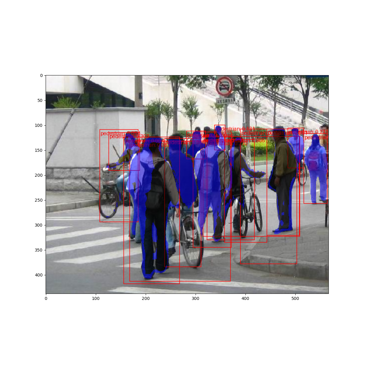
So after one epoch of training, we obtain a COCO-style mAP > 50, and a mask mAP of 65.

But what do the predictions look like? Let’s take one image in the dataset and verify

import matplotlib.pyplot as plt

from torchvision.utils import draw_bounding_boxes, draw_segmentation_masks


image = read_image("data/PennFudanPed/PNGImages/FudanPed00046.png")
eval_transform = get_transform(train=False)

model.eval()
with torch.no_grad():
    x = eval_transform(image)
    # convert RGBA -> RGB and move to device
    x = x[:3, ...].to(device)
    predictions = model([x, ])
    pred = predictions[0]


image = (255.0 * (image - image.min()) / (image.max() - image.min())).to(torch.uint8)
image = image[:3, ...]
pred_labels = [f"pedestrian: {score:.3f}" for label, score in zip(pred["labels"], pred["scores"])]
pred_boxes = pred["boxes"].long()
output_image = draw_bounding_boxes(image, pred_boxes, pred_labels, colors="red")

masks = (pred["masks"] > 0.7).squeeze(1)
output_image = draw_segmentation_masks(output_image, masks, alpha=0.5, colors="blue")


plt.figure(figsize=(12, 12))
plt.imshow(output_image.permute(1, 2, 0))

<matplotlib.image.AxesImage object at 0x7f823da36b90>

The results look good!

Wrapping up

In this tutorial, you have learned how to create your own training pipeline for object detection models on a custom dataset. For that, you wrote a torch.utils.data.Dataset class that returns the images and the ground truth boxes and segmentation masks. You also leveraged a Mask R-CNN model pre-trained on COCO train2017 in order to perform transfer learning on this new dataset.

For a more complete example, which includes multi-machine / multi-GPU training, check references/detection/train.py, which is present in the torchvision repository.